Multiverse 2.357

IBM has quantum computers online and available for the general public to use for free. We’re going to look at interacting with them through the online interface, then we’ll dive in and take a look at writing and running programs using their Python framework called Qiskit. There are other great frameworks out there to use, and we’ll get to those, but this is a great place to start.

The first thing to do is to make yourself an account at the IBM Q site so that we can use their quantum computers. Usually people are eager to start playing around with these mysterious devices, but when you get a chance, explore the detailed documentation and learn what they have to offer.

We’re basically programming against a quantum computer at the assembly language level or just higher, in fact you might notice a reference to ‘qasm’ which stands for quantum assembly.

IBM’s architecture use electrons on silicon wafer technology kept at supercool temperatures, which are put into quantum states by injecting microwaves. But we’re not programming at the machine level, so the types of gate operations we do would work on any general purpose quantum computer even though the syntax would vary. We are constructing circuits by applying gates to our qubits. That’s the level we’re programming at.

Your IBM Q Account

The IBM Q website has documentation and tutorials, along with a quantum circuit tool that lets you visually construct programs to run on their machines. Create the number of qubits (those horizontal lines) that you need, and drag-n-drop gates onto them. If you have experience in classical computer hardware design, try to relate this to designing logic with unary and binary gates like AND, NAND, NOT and XOR.

Notice that one of the choices on the left is to display the quantum assembly (qasm) code corresponding to the circuit tool on the right. In this case, we are creating two quantum registers, q[0] and q[1], along with two classical ones indicated by the label c2. We then apply a Hadamard gate (we’ll explain more about this later) to the first quantum register, q[0] and a CNOT gate from the first quantum register to the second. Don’t worry about what these do for now, we just want to see what a quantum circuit looks like.

Finally we applied two measure operations, which is the only way we can read the values. This is always the last operation, as it collapses the quantum probabilistic state into a specific one, like opening the box to observe that Schrödinger’s cat is alive or dead. The measurement operation copies the observed values from our two quantum registers to the classical registers as actual zeros or ones.

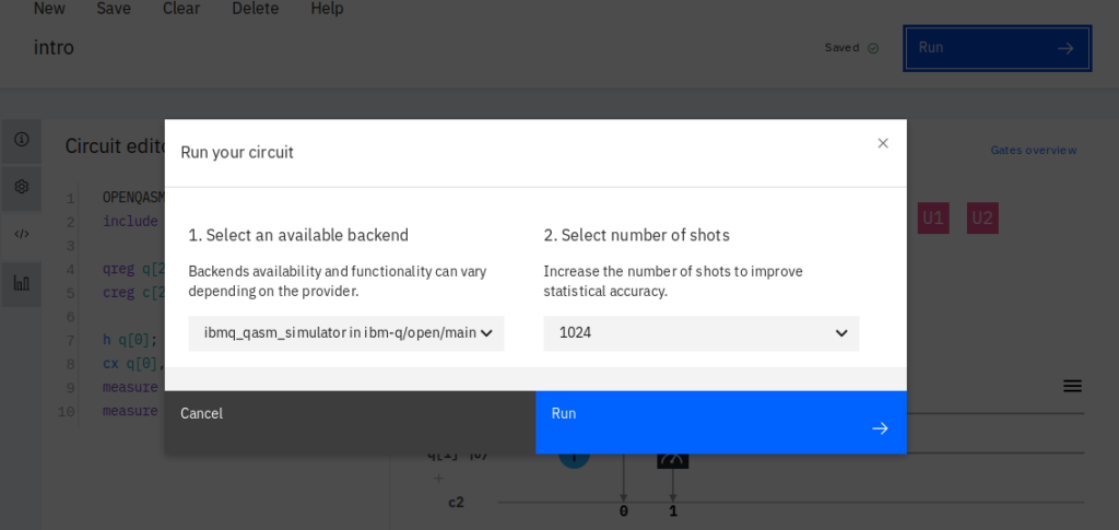
We can save and run our “quantum program” represented by this visual depiction of the circuit. The choices are shown above: which backend provider we wish to use, and how many times to run this. We need to run quantum programs many times since they are not deterministic, they are probabilistic so there is no guarantee that an individual outcome is the one we consider to be “correct”.

As you can see, we got almost 49% of the 1024 results measuring both values as zeros, and just over 51% of the results showing both values being ones. We didn’t get any results showing 0 and 1, or 1 and 0, but sometimes we would. This is not just due to the probabilistic nature of quantum algorithms, but also to the sensitivity of qubits with respect to “noise”; error rates in current quantum computers are high.

A Few Basic Gates

There are more gates, but let’s look at just a few so we have have enough background to write some simple programs. We saw three gates earlier, the Hadamard gate, the CNOT gate, and our old friend the Measure operation.

The first gate we should look at is the X gate that acts on a single qubit, analogous to a NOT in the logic gates of classical computers – it flips the value of the qubit. That is, it takes a |0> to a |1> and it takes a |1> to a |0>. In qasm it’s written as x.

x|0> = |1>
x|1> = |0>

Next up, the conditional NOT, or CNOT gate, which operates on two qubits and is sort of analogous to the XOR logic in the classical world. The CNOT acts upon a target qubit based on the value of a control qubit. The control qubit determines whether or not the target qubit is flipped. If the control bit is |0> the target qubit is not flipped, but if the control qubit is |1> then the target qubit is flipped. This is written as cx(source, target) in qasm.

The Hadamard gate, written as h(target) in qasm, puts qubits into a state of superposition. Think of a coin laying flat as showing either heads or tails (representing zero or one) and imagine the Hadamard gate putting the coin into a state of spinning, where it has both possible values until the spinning is stopped.

The measure operation is the one that stops the coin from spinning, to reuse the previous analogy. Qubits begin in a state of |0> and often the first gate applied is a Hadamard gate, to put them into a state of superposition. Similarly we often see the last operation applied is a measure, since it is no longer useful for computations after that.

In our introductory quantum circuit constructed above, we took two qubits, each starting in a |0> state, and put the first into a state of superposition using the Hadamard gate. We then applied a CNOT gate, from the first to the second. This means that if the first qubit is measured to be zero, the second one will be unchanged. And since it started as zero, it will remain so. If the first qubit is measured to be a one, it flips the value of the second, causing it to change from zero to one.

So either they are both measured to be zero, or they are both measured to be one. This is an important result called quantum entanglement, or as Einstein called it, “spooky action at a distance.” This is an important building block that we will see again.

Entanglement does not make a lot of sense to me from a physics perspective, because the values are not decided by the entangled particles before they are separated. The values are also not communicated to each other when one particle is observed, and yet measuring one value collapses the possible values of the other instantly, regardless of distance. Since I don’t understand it, I won’t attempt to explain it.

Fortunately entanglement totally makes sense if you ignore the physics and just look at the math. But doing so means I have to admit that I’ve oversimplified pretty much everything so far. For example, applying the Hadamard gate to |0> is not the same as applying it to |1>. Qubits are not simply representing a spectrum of real values from zero to one inclusive, but in truth represent imaginary numbers. So for now just trust me, the math makes sense if explained, but I would prefer to actually write a program next instead of offering up yet another post on background information.

So next we’re going to get our hands dirty and actually take a look at the python framework called Qiskit. It allows us to write programs instead of using the visual circuit builder. This circuit builder is nice, but quickly becomes insufficient as we explore non-trivial programs.